

In biological research, fluorescent proteins (FPs) are widely used in fluorescence microscopy. FPs are genetically encoded fluorophores, which are produced by cells after a noninvasive transfection. These proteins are utilized as markers and bio-sensors to study biological processes in living cells at high spatial and temporal resolution. Currently, many different types of FPs exist, comprising different spectral properties (i.e. colors), fluorescence lifetime characteristics, photo switching behavior, brightness, pH sensitivity, etc.
New FPs are continuously being developed in order to optimize their properties for specific applications. The fluorescence lifetime is an excellent parameter to use as selection marker in a screening for optimized FPs. The fluorescence lifetime is correlated with the quantum yield and thus the intrinsic brightness. In contrast, the fluorescence intensity is correlated with the brightness and protein concentration. Therefore, when only fluorescence intensity is used for screening, the selection will be biased towards samples with a higher concentration. Also the effects of environment can affect the fluorescence lifetime, e.g. the pH and chloride ions. A main application where the fluorescence lifetime is a key molecular property, is in Förster Resonance Energy Transfer (FRET) based molecular biosensors. Here changes in molecular interactions or conformation can be directly observed by measuring the donor life-time and changes thereof.
We developed a multi-position fluorescence lifetime imaging (FLIM) screening method to screen for bright FPs. However, this method can be applied to any experiment in which the fluorescence lifetime is an important parameter. To be able to test many different FP mutants (samples), an efficient acquisition and data processing workflow is paramount to obtain high quality and reproducible data with high throughput. The LIFA system, with the aid of MATLAB® and ImageJ [1], can be utilized to set up such an automated screening and characterization approach, allowing full flexibility.
Researchers at the University of Amsterdam developed a multi-position fluorescence lifetime imaging (FLIM) screening method to screen for bright FPs. However, this method can be applied to any experiment in which the fluorescence lifetime is an important parameter.
AUTOMATED MULTI-POSITION FLIM ACQUISITION WITH MATLAB
Lambert Instruments has provided a versatile library of interface functions (API) that allows direct communication with the LIFA software via MATLAB, in order to control the LIFA camera (Fig. 1A) and the microscope (Fig. 1B). With the aid of this API, a custom made MATLAB graphical user interface (GUI) was developed that allows multi-position acquisition.
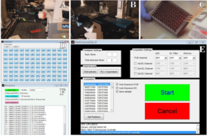
Figure 1. Automated 96-well lifetime acquisition. The LIFA camera (A) and microscope (B) iterate over a 96 well plate (C). Each well can be selected or deselected by using the well selector (D). The selected coordinates are loaded into the MATLAB GUI and specific excitation and emission filters can be selected together with auto-exposure and output file settings (E). Finally, lifetime files (fli) are exported to a large TIF hyperstack (F) for further processing with ImageJ.
In this example, each well in a 96-well plate contains mammalian cells transfected with DNA encoding a different FP (Fig. 1C). Prior to the multi-position acquisition, specific wells can be selected or deselected by using a secondary MATLAB GUI (Fig. 1D). After this, a text file and an Excel file are exported, both only containing the selected wells. The Excel file comprises the well names, the well coordinates and also contains a column where the user can add metadata about each well (e.g. name of FP).
Before acquisition is started, it is possible to set other parameters within the LIFA software and to acquire a calibration lifetime measurement. Furthermore, options to use auto-exposure and to choose the type of output files that will be stored for later processing are present (i.e. calculated lifetime images, raw phase images or DC images) (Fig. 1E). After the coordinate file is loaded and acquisition is commenced, the MATLAB script iterates over all coordinates, taking phase stacks and storing the selected output files. Each lifetime file (.fli) comprises four channels, including lifetime data and the fluorescence intensity data. The files also contain metadata about the position, exposure time and reference lifetime. Using another secondary custom made MATLAB GUI, all the fli-files are imported using the Bio-Formats [2] package for MATLAB and the image data and metadata are extracted. Subsequently, all the raw images are exported to an ImageJ TIF hyperstack (Fig. 1F) that can be directly processed with ImageJ. The reference lifetime, the exposure time for each well as well as the information previously stored in the Excel file are added to the metadata for later use. This helps the user to keep track of the wells and their metadata during processing.
DATA PROCESSING AND VISUALIZATION USING IMAGEJ
In order to process the large quantities of lifetime data, several ImageJ macros were written that can be easily operated by any user. The user sets several parameters before processing, including smoothing and also thresholding (Fig. 2A). The macro generates three files: an ImageJ TIF stack (Fig. 2B), a 96-well layout figure (Fig. 2C), and a numerical table. The 96-well layout displays the mean phase lifetime, mean modulation lifetime and mean intensity of all wells and will therefore quickly indicate the wells of interest. Each multi-panel FLIM figure of the ImageJ TIF stack gives a detailed FLIM analysis per well. The multi-panel FLIM figure (Fig. 2D) displays the intensity image in grayscale (I) and the following panels for the phase and modulation lifetimes: a false color image (II), a false color image with intensity overlay (III), a lifetime histogram (IV), a scatterplot of the lifetime versus the intensity (V). Finally, the polar plot (VI) is shown together with the scatterplot of phase versus modulation lifetime (VII). In addition, each multi-panel FLIM figure also includes metadata i.e. the exposure time, well number, the user added metadata, and the original file name.
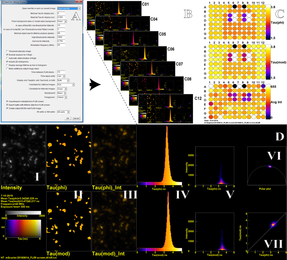
Figure 2. An ImageJ macro (A) allows to set several processing and display parameters and generates a TIF stack with display figures for all wells present in the hyperstack (B) and a 96-well layout with the mean lifetime data (C). A detailed FLIM analysis from one well (D), the TIF stack (B) containing an extensive FLIM analysis of each well. The multi-panel D contains: grayscale (I), lifetime false color images (II), lifetime false color image with intensity overlay (III), a lifetime histogram (IV), a scatterplot of the lifetime versus the intensity (V), the polar plot (VI) and a scatterplot of phase (phi) versus modulation (mod) lifetime (VII).
The wells in Figure 2 are measurements of newly developed mScarlet red FP variants [3] in mammalian cells. The measurements are highly reproducible; in figure 2 only 4 variants have been used and only 4 colors appear in the phase and modulation lay-out in figure 2C. The lifetime histograms (Fig. 2D IV) of different wells that are transfected with the same FP are very similar. The width of the histograms mainly reflects the variability across cells, and is much narrower for measurements performed on solutions with purified FPs. By using this approach we found a monomeric red FP variant, named mScarlet, with the highest fluorescence lifetime and quantum yield up to date. As mentioned before, this pipeline can also be utilized for other screening and characterization applications where fluorescence lifetime is an important readout, for example optimization of FRET based biosensors, testing of agonist and antagonist dose dependency and pH sensitivity of fluorescent proteins. Taken together, using this pipeline, it is possible to screen many constructs and conditions in a fast automated and user-friendly way, yielding robust and highly reproducible results.
ACKNOWLEDGEMENTS
Lambert Instruments (Johan Herz MATLAB API scripting), NWO-STW grant 12149, NWO CW-Echo grant 711.01.01812, NWO ALW-VIDI grant 864.09.015 and Nikon Netherlands
REFERENCES
1. Schneider, C. A.; Rasband, W. S. & Eliceiri, K. W. (2012), NIH Image to ImageJ: 25 years of image analysis, Nature methods 9(7): 671-675.
2. Melissa Linkert, Curtis T. Rueden, Chris Allan, Jean-Marie Burel, Will Moore, Andrew Patterson, Brian Loranger, Josh Moore, Carlos Neves, Donald MacDonald, Aleksandra Tarkowska, Caitlin Sticco, Emma Hill, Mike Rossner, Kevin W. Eliceiri, and Jason R. Swedlow (2010) Metadata matters: access to image data in the real world. The Journal of Cell Biology, Vol. 189no. 5777-782.
3. Daphne S. Bindels, Lindsay Haarbosch, Laura van Weeren, Marten Postma, Katrin E Wiese, Marieke Mastop, Sylvain Aumonier, Guillaume Gotthard, Antoine Royant, Mark A. Hink and Theodorus W.J. Gadella Jr. mScarlet: a novel bright monomeric red fluorescent protein for cellular imaging. Nature Methods (2016)
The spectrally-resolved Lambert Instruments FLIM Attachment (LIFA) is an imaging system for fluorescence microscopy that preserves the information required to determine the position, spectrum, and lifetime of the observed fluorescence. This is done by combining several modular components. These consist of the typical LIFA (modulated intensified CCD camera, modulated LED excitation) and a prism-based imaging spectrograph.
The data below were obtained with the Lambert Instruments FLIM Attachment (LIFA), either widefield (with LED light; 468nm peak) or confocal (with spinning disk CSU10 and 470nm-diode laser). The fluorescence lifetime images are generated at 2 different z-positions, z1 and z2. Snapshots of several z-positions are shown, as well as movies through even more.
SPECTRALLY RESOLVED
2D IMAGE
CONFOCAL
(SPINNING DISK)
WIDEFIELD
(LED)
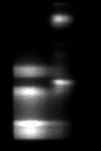
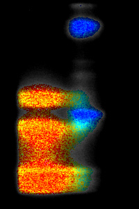
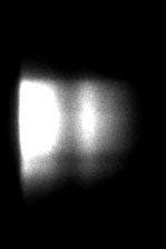
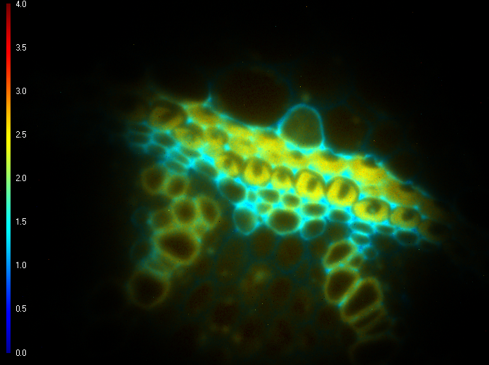
The spectrally resolved images show one line (y-axis) out of the 2D intensity image of typical dicot root. The emission wavelengths at the x-axis start at 515 nm. The fluorescence lifetime is shown in pseudo colors. The higher wavelength components have a shorter lifetime (blue) than the short wavelength components (red).
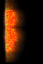
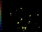
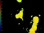
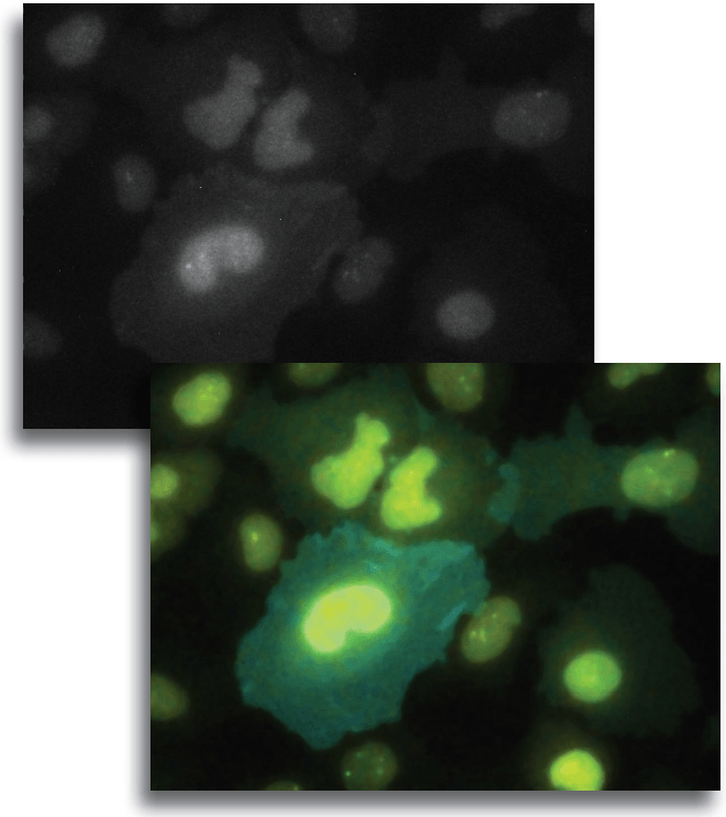
SPECTRALLY RESOLVED GFP TRANSFECTED CELLS (DONOR ONLY)
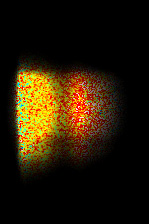
SPECTRALLY RESOLVED GFP-RFP TRANSFECTED CELL (FRET)
LIFETIME (PSEUDOCOLORS)
INTENSITY (GRAYSCALE)
The spectrally resolved images show one line (y-axis) out of a sample of GFP transfected cells or GFP-RFP transfected cells. The emission wavelengths at the x-axis start at 515 nm; the first peak is the GFP emission peak and the second the RFP emission peak. The fluorescence lifetime is shown in pseudo colors. In the FRET sample (GFP-RFP) the fluorescence lifetime of the GFP has decreased from 2.3 ns (red) to 2.0 ns (yellow).
The differences in lifetime could be due to the fact that the diode laser has one excitation wavelength, exactly 470 nm, while the LED has a range of wavelengths for which we used the emission band pass filter of 465-495 nm.
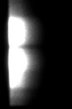
Total Internal Reflection Fluorescence (TIRF) microscopy facilitates extremely high-contrast visualization and thereby high sensitivity of fluorescence near the cover glass. Typically, the optical section adjacent to the cover glass is about 100 nm. TIRF does not disturb cellular activity, thus enabling tracking of biomolecules, and the study of their dynamic activity and interactions at the molecular level. TIRF enables the selective visualisation of processes and structures of the cell membrane and pre-membrane space like vesicle release and transport, cell adhesion, secretion, membrane protein dynamics and distribution or receptor-ligand interactions. The unique combination of TIRF and frequency domain FLIM makes it possible to measure lifetimes of, for instance, small focal adhesions near the cover glass.
TIRF
WIDEFIELD
LIFETIME (PSEUDOCOLORS)
INTENSITY (GRAYSCALE)
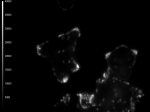
These cells (kindly provided by Ms. S.E. Le Devedec, Leiden University, The Netherlands) express dSH2-GFP in small focal adhesions as well as in the nuclei as shown by widefield microscopy. However, by the use of TIRF only fluorescence close to the coverslip is obtained, thus only the focal adhesions are excited.
Fluorescence lifetime images give a more accurate measurement in TIRF mode, as out of focus light is emitted from the average lifetime in the focal adhesions.
The images shown here are taken with the Nikon TE2000-U widefield microscope with white-TIRF illuminator, combined with the Lambert Instruments Fluorescence lifetime imaging Attachment (LIFA). As light source the modulated LED of 468nm 3W was used and as demonstrated here enough intensity was generated to obtain fluorescence lifetime images with TIRF.
TIRF
WIDEFIELD
LIFETIME (PSEUDOCOLORS)
INTENSITY (GRAYSCALE)
Cells (kindly provided by Ms. S.E. Le Devedec, Leiden University, The Netherlands) expressing dSH2-GFP in small focal adhesions as well as in the nuclei.
The images shown here are taken with the Olympus TIRFM (laser-TIRF), combined with the Lambert Instruments FLIM Attachment (LIFA). As light source the modulated diode laser of 473 nm 20 mW was used and as demonstrated here enough intensity was generated to obtain fluorescence lifetime images with TIRF.
TIRF
LIFETIME (PSEUDOCOLORS)
INTENSITY (GRAYSCALE)
Cells (kindly provided by Ms. S.E. Le Devedec, Leiden University, The Netherlands) expressing dSH2-GFP in small focal adhesions as well as in the nuclei.
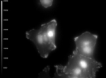
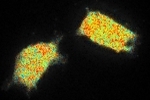
Information processing and storage in the brain involves fast communication between neurons. In the central nervous system a neuron can be connected to up to thousands of other neurons through brain synapses, specialized junctions where the axon of one neuron meets the dendrite of another neuron (two examples are shown by red arrows on the images below). Over time, the efficacy of synaptic transmission can vary depending upon synaptic activity, a mechanism called synaptic plasticity that is largely responsible for learning and memory. During synaptic plasticity, proteins can be specifically accumulated at synapses through protein-protein interactions. The group of Daniel Choquet at the University of Bordeaux Segalen aims at gaining a better understanding of protein accumulation at synapses to unravel the molecular mechanisms underlying memory storage in the brain.
The data below were obtained with the Lambert Instruments FLIM Attachment (LIFA), either widefield (with LED light; 468nm peak) or confocal (with spinning disk CSU10 and 470nm-diode laser). The fluorescence lifetime images are generated at 2 different z-positions, z1 and z2. Snapshots of several z-positions are shown, as well as movies through even more.
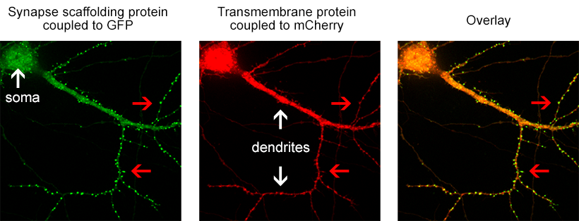
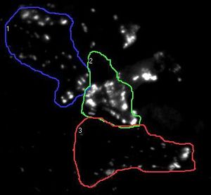
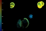
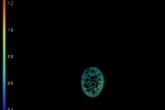
Figure 1. the donor and acceptor proteins co-localize in neurons.
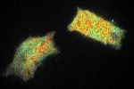
Using primary neuronal cultures from rat hippocampus, PhD student Anne-Sophie Hafner studied the localization of interactions between two specific neuronal proteins; an intracellular scaffolding protein and a transmembrane receptor. She transfected neurons with DNA encoding a synaptic protein coupled to Green Fluorescence Protein (GFP) (donor, green image) and a transmembrane protein coupled to mCherry (acceptor, red image). She used the Lambert Instruments FLIM Attachment (LIFA) on a confocal spinning disk to monitor GFP lifetime with or without acceptor proteins. During the experiment, cells are first imaged through the spinning disk to ensure the presence and co-localization of the donor and acceptor proteins. As shown in figure 1, both proteins are co-localized in all cell compartments, the synapse scaffolding protein being enriched in synapses. Then, the cells are imaged on the LIFA attached TRiCAM, to generate the FLIM image (lifetime color coded for each pixel, last image).
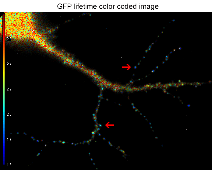
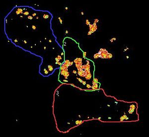
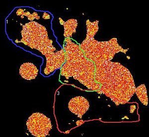
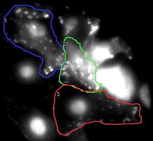
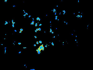
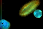
Figure 2. the donor and acceptor protiens interact specifically in synapses.
An example lifetime image of a neuron is shown in Figure 2. In the soma and dendrites, GFP lifetime is high (i.e. no interaction between the proteins of interest), and not different compared to GFP lifetime without acceptor fluorophore which stands around 2.6 nanoseconds. In contrast, GFP lifetime in synapses is dramatically decreased in presence of the acceptor protein to a mean value of 1.9 nanoseconds (i.e. the proteins of interest are interacting specifically in synapses). The Lambert Instruments FLIM technology allowed us to show and quantify for the first time the synapse specific interaction of the two proteins of interest.
ACKNOWLEDGEMENTS
Data courtesy of Anne-Sophie Hafner, Interdisciplinary Institute for Neuroscience, University of Bordeaux Segalen, France
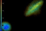
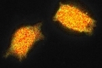
Confocal imaging on a widefield fluorescence microscope can now be done in combination with frequency-domain fluorescence lifetime imaging microscopy (FLIM). The increased spatial resolution in the z-direction results in lifetime images with enhanced contrast as the detection of out-of-focus emission is reduced significantly. This allows you to see differences in fluorescence lifetime e.g. between the cell membrane and the cytoplasm.
The data below were obtained with the Lambert Instruments FLIM Attachment (LIFA), either widefield (with LED light; 468nm peak) or confocal (with spinning disk CSU10 and 470nm-diode laser). The fluorescence lifetime images are generated at 2 different z-positions, z1 and z2. Snapshots of several z-positions are shown, as well as movies through even more.
Z1
Z2
CONFOCAL
(SPINNING DISK)
WIDEFIELD
(LED)
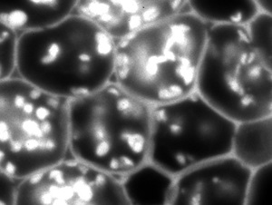
These images show different pollen grains: the lifetime in pseudo colours and the intensity in grey scale. Because of the pinholes in the spinning disk, the exposure time is higher with confocal imaging. In this image 220 ms exposure time per phase step was taken for the confocal image versus 195 ms for the widefield (LED light). However, when a diode laser with higher power is used, the exposure time can be shortened.
Z1
Z2
CONFOCAL
(SPINNING DISK)
WIDEFIELD
(LED)
These images show YFP-transfected mammalian cells and were taken with 12 phase steps of each 400 ms for the confocal, versus 70 ms for the widefield image. The calculated lifetimes are 2.34 ns (z1) and 2.42 ns (z2) in the confocal images, versus 2.58 ns (z1) and 2.57 ns (z2) in the widefield images.
The differences in lifetime could be due to the fact that the diode laser has one excitation wavelength, exactly 470 nm, while the LED has a range of wavelengths for which we used the emission band pass filter of 465-495 nm.
Fluorescence lifetime can be recorded for every pixel in the image simultaneously with a time-domain FLIM camera. This method requires an intensified camera, a pulsed laser and a widefield fluorescence microscope. This is typically more cost-effective than alternative methods that need a confocal set-up.
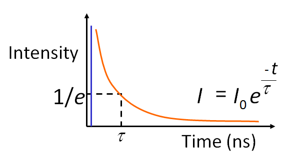
One of the most popular methods for fluorescence lifetime imaging microscopy (FLIM) is time-correlated single photon counting (TCSPC). This method requires a confocal microscope with a pulsed laser and a photomultiplier tube (PMT). The sample is briefly illuminated by a laser pulse after which the PMT counts the number of emitted fluorescence photons. The intensity I of the fluorescence emission decays exponentially after the laser pulse has excited
the sample:
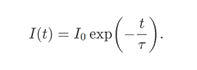
The fluorescence lifetime τ𝜏 quantifies the rate of decay of the fluorescence light. By scanning the sample with a focused laser beam, TCSPC systems can construct a fluorescence lifetime image of the sample one pixel at a time.
As an alternative to TCSPC on a confocal microscope, Lambert Instruments has developed a new system that brings time-domain FLIM to widefield microscopes. By carefully timing the exposure of the camera in the subnanosecond range, a light pulse profile of the fluorescence light can be captured. This method requires a pulsed laser and an intensified camera to record the raw data. Custom Lambert Instruments software then processes this data to automatically calculate the fluorescence lifetime.
SET-UP
Images were recorded with the LIFA-TD, which has a CCD camera with a fiber-optically coupled image intensifier. The image intensifier boosts the incoming light levels and it can achieve gate widths of less than 3 ns. A 485 nm pulsed laser (Picoquant LDH-D-C-485 laser head with a PDL 800-B laser driver) with a fiber-optical output was coupled into a widefield fluorescence microscope (Nikon Eclipse Ti) to provide 85 ps excitation pulses.
METHODS
The set-up was calibrated by recording the light pulse profile of the laser by placing a highly reflective material in the sample holder of the microscope. Next, the fluorescence decay profile of a convallaria (lily of the valley) sample was recorded. The fluorescence lifetime is determined by correlating the fluorescence emission to the light pulse profile.
RESULTS
Figure 1 shows the fluorescence lifetime of a convallaria sample overlayed on the original image. The LIFA-TD is able to detect the small variations in fluorescence lifetime between different parts of the sample, stained with different dyes.
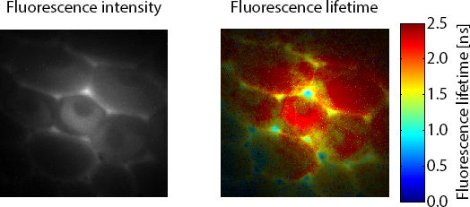
Figure 1: Fluorescence intensity (left) recording of convallaria sample and corresponding fluorescence lifetimes (right) overlayed on the original image.
CONCLUSION
Time-domain fluorescence lifetime imaging microscopy can be done on a widefield fluorescence microscope by using an intensified camera and a pulsed laser. The LIFA-TD is an entry-level FLIM system that offers an integrated solution.
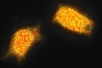
Recording images of living organisms at high frame rates with a fluorescence microscope is challenging. High-speed imaging requires a considerable light intensity, because at high frame rates the image sensor is exposed to light very briefly. During that short period of time, enough light needs to be captured to obtain a clear image. Normally, this is achieved by increasing the intensity of the illumination. Because the more light bounces off the object, the more light reaches the camera. But when studying fluorescence or chemiluminescence, the object itself emits light and increasing the intensity of the emitted light is often not possible. In such a situation, the solution is to increase the intensity of the light that is detected by the camera.
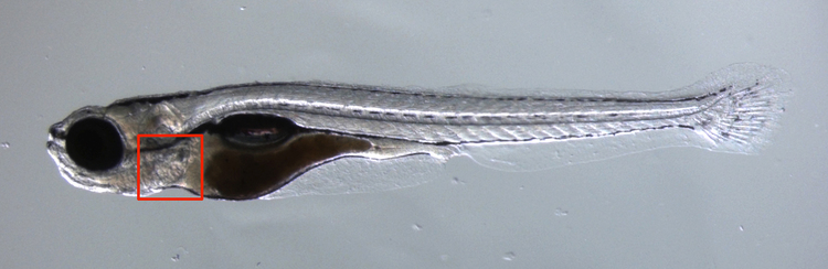
Figure 1. Photo of a zebrafish. The heart is located inside the red square.
IMAGING THE CARDIOVASCULAR SYSTEM OF A ZEBRAFISH
At the Max Planck Institute for Heart and Lung Research in Bad Nauheim (Germany), the cardiovascular system of the zebrafish is studied. The transparency of the zebrafish (figure 1) and its experimental advantages make it an ideal scale model of the human cardiovascular system.
To study the blood flow in a zebrafish, the red blood cells are labeled with the fluorescent protein DsRed. The intensity of the fluorescent light is limited by the finite number of fluorescent proteins attached to the red blood cells. Also, the direction in which the light is emitted is random, which further decreases the amount of light reaching the camera. A low light intensity is not necessarily problematic. Increasing the exposure time to capture sufficient light is a well known method for imaging dim objects that are stationary. However, using the same method on a moving object results in blurred images.
When imaging a living zebrafish, its internals are moving. The heart rate of a zebrafish is approximately 175 bpm, or nearly 3 beats per second. To capture each phase of the heart beat requires a high frame rate, because otherwise the images will be distorted by motion blur. This means the image sensor is being exposed to the dim fluorescent light very briefly. Increasing the amount of fluorescent light by increasing the intensity of the excitation light is not an option, as this would harm the fish.
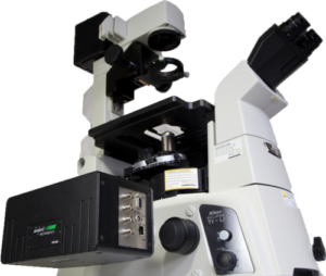
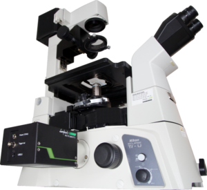
Figure 2. HiCAM attached to fluorescence microscope.
EXPERIMENTAL SETUP
The zebrafish is studied with a fluorescence microscope with high-speed camera system mounted to it (figure 2). The fish is fixated in a gel and illuminated from below. Fluorescent light from the DsRed protein is emitted from the red blood cells. This light is emitted in every direction, some of it traversing the optical path of the laser in the opposite direction. But instead of being reflected back towards the light source, the fluorescent light is directed towards a camera through a dichroic mirror. Any scattered excitation light is reflected by the dichroic mirror. An optical filter removes any background light and only transmits light at the wavelength emitted by fluorescence of the red blood cells.
An image sensor will capture the incoming fluorescent light. At frame rates of hundreds or thousands of frames per second, the exposure time for each frame is in the order of several milliseconds to fractions of milliseconds. Electron-Multiplied CCD (EMCCD) sensors have a light sensitivity that is good enough to capture the dim fluorescent light. But they can only achieve frame rates up to approximately 100 fps at full resolution, which is not enough for the application at hand. CMOS sensors can operate at higher frame rates, up to thousands of frames per second at full resolution. However, during the short exposure time of each frame, a regular high-speed CMOS sensor is not able to record a sufficient amount of light to achieve a reasonable signal-to-noise ratio.
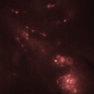
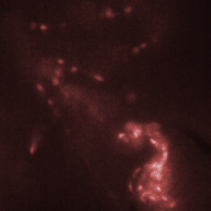
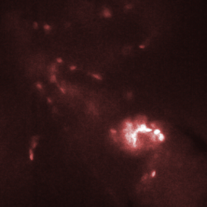
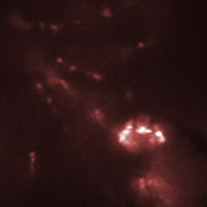
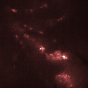
Figure 3. Red blood cells in the heart of a zebrafish (bottom right corner of images) are transported from one chamber to the next chamber (a-c) and into the aorta (e). Images shown here were recorded with an interval of 25 ms between them. Recording was done at 2000 fps with an exposure time of 500 us.
ADVANTAGES OF THE HICAM
The HiCAM achieves both the required light sensitivity and the high frame rates by combining a high-speed CMOS sensor with an image intensifier. The image intensifier increases the number of detected photons by several orders of magnitude. This way, it is possible to record the blood flow in a zebrafish at 2000 frames per second. Figure 3 shows the flow of red blood cells through the cardiovascular system of the zebrafish.
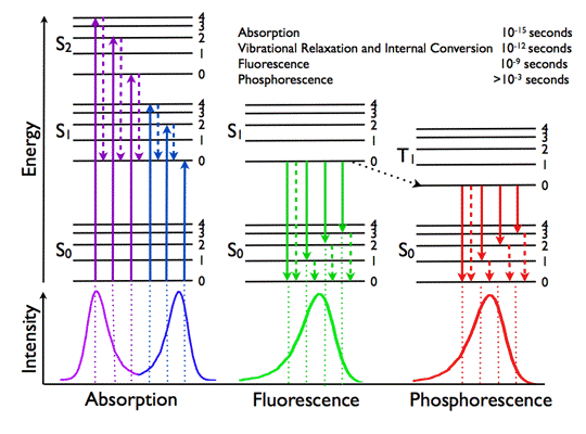
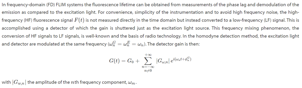
In this article the first principles of frequency domain (FD) fluorescence lifetime imaging microscopy (FLIM) are further explained through use of equations. Although these principles not necessary for the execution of basic lifetime measurements, a thorough understanding provides the groundwork that enables deeper insight into your results and into the possibilities of FD lifetime imaging.
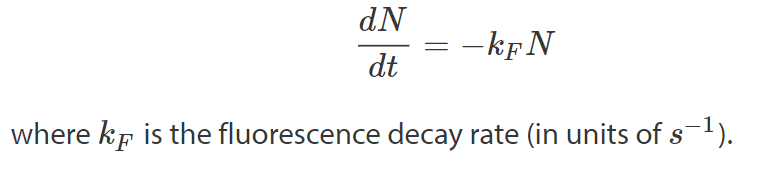
Fluorescence Lifetime
For an ensemble of fluorescent molecules the rate at which molecules decay from the excited state to the ground state (cf. Fig.1) is proportional to the number of excited state molecules N:
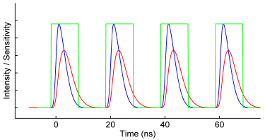
Homodyne Detection
A selection of papers papers based on Lambert Instruments FLIM systems is maintained here.
The following is a selection of books and papers on FLIM technology:
BOOKS / REVIEWS:
Gadella TW Jr., FRET and FLIM techniques, 33. Elsevier, ISBN-13: 978-0080549583. (Dec 2008) 560 pages. Elsevier link
Periasamy, A & Clegg RM, FLIM Microscopy in Biology and Medicine. Chapman & Hall/CRC, 1st edition, ISBN-13: 978-1420078909. (Jul 2009) 368 pages. Amazon link
Lakowicz JR. Principles of fluorescence spectroscopy, 3rd edition, ISBN-13: 978-0387312781 . Springer, 3rd edition (Sep 2006) 954 pages. Amazon link
Van Munster EB, Gadella TW Jr. Fluorescence lifetime imaging microscopy (FLIM). Review. Adv Biochem Eng Biotechnol. (2005) 95:143-75. Pubmed link
BOOKS; FLUORESCENT PROTEINS / CELL BIOLOGY:
Sullivan KF, Fluorescent Proteins, 2nd Edition Volume 85. Academic Press, ISBN-13: 978-0123725585. (Dec 2007) 660 pages. Amazon link
Sullivan KF, Kay SA, Wilson L, Matsudaira PT,Green Fluorescent Proteins, Volume 58. Academic Press, ISBN-13: 978-0125441605. (1998) 386 pages. Amazon link
PAPER MULTIFREQUENCY:
Squire A, Verveer PJ, Bastiaens PIH, Multiple frequency Fluorescence lifetime imaging microscopy. Journal of Microscopy, (2000) 197(2):136-149. Pubmed link
PAPER PHASE STEP ORDER:
Van Munster EB, Gadella TW Jr, Suppression of photobleaching-induced artifacts in frequency-domain FLIM by permutation of the recording order. Cytometry A. (2004) 58(2):185-94. Pubmed link
PAPERS POLAR PLOT:
Redford GI, Clegg RM, Polar plot representation for frequency-domain analysis of fluorescence lifetimes. Journal of Fluorescence (2005) 15(5):805-815. Pubmed link
Clayton AHA, Hanley QS, Verveer PJ. Graphical representation and multicomponent analysis of single-frequency fluorescence lifetime imaging microscopy data. Journal of Microscopy (2004) 213(1):1-5. Pubmed link
PAPERS TIRF-FLIM:
Valdembri D, Caswell PT, Anderson KI, Schwarz JP, König I, Astanina E, Caccavari F, Norman JC, Humphries MJ, Bussolino F, Serini G, Full Text
What is the Fluorescence lifetime?
The fluorescence lifetime – the average decay time of a fluorescence molecule’s excited state – is a quantitative signature which can be used to probe structure and dynamics at micro- and nano scales. FLIM (Fluorescence Lifetime Imaging Microscopy) is used as a routine technique in cell biology to map the lifetime within living cells, tissues and whole organisms. The fluorescence lifetime is affected by a range of biophysical phenomena and hence the applications of FLIM are many: from ion imaging and oxygen imaging to studying cell function and cell disease in quantitative cell biology using FRET.
For fluorescent molecules the temporal decay can be assumed as an exponential decay probability function:
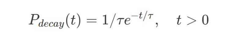
where t is time and τ is the excited state lifetime.
More complex fluorophores can be described using a multiple exponential probability density function:
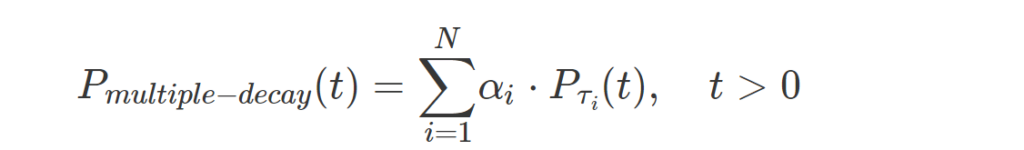
where t is time, τi is the lifetime of each component and αi is the relative contribution of each component.
Why Measure Fluorescence Lifetime?
A key advantage of the fluorescence lifetime is that it is a basic physical parameter that does not change with variations in local fluorophore concentration and is independent of the fluorescence excitation. Hence the lifetime is a direct quantitative measure, and its measurement – in contrast to e.g. the recorded fluorescence intensity – does not require detailed calibrations. Excited state lifetimes are also independent of the optical path of the microscope, photobleaching (at least to first order), and the local fluorescence detection efficiency.
The fluorescence lifetime does change when the molecules undergo de-excitation through other processes than fluorescence such as dynamic quenching through molecular collisions with small soluble molecules like ions or oxygen (Stern-Volmer quenching) or energy transfer to a nearby molecule through FRET. As a result the fluorophores (in the excited state) lose their energy at a higher rate, causing a distinct decrease in the fluorescence lifetime. The measured rate of fluorescence is actually a summation of all of the rates of de-excitation. In this way the fluorescent lifetime mirrors any process in the micro-environment that quenches the fluorophores; and spatial differences in the amount of quenching reveals itself as contrast in a lifetime image.

5th floor,
Leonard Springerlaan 19
9727KB Groningen
The Netherlands